Project context
Drexel University ran Yellowstone field courses to introduce high school students to the geosciences and environmental science. Students learned remote sensing by scanning geysers with an iPad and by walking around the geysers with a Velodyne LiDAR puck mounted on a handheld pole.
The course leader's long-term aim was to rescan the same geysers each year and compare the point clouds to measure geyser change over time. Funding for the course ended after two seasons, so the record covers 2022 and 2023 only.
My role
- Processed the 2023 Velodyne capture files with SLAM to recover the sensor path and build a map
- Aggregated the frames into a single point cloud and cleaned it for modelling
- Generated the DEM and the 3D surface models
- Wrote a step-by-step processing protocol so later cohorts could repeat the workflow
3D Surface Model
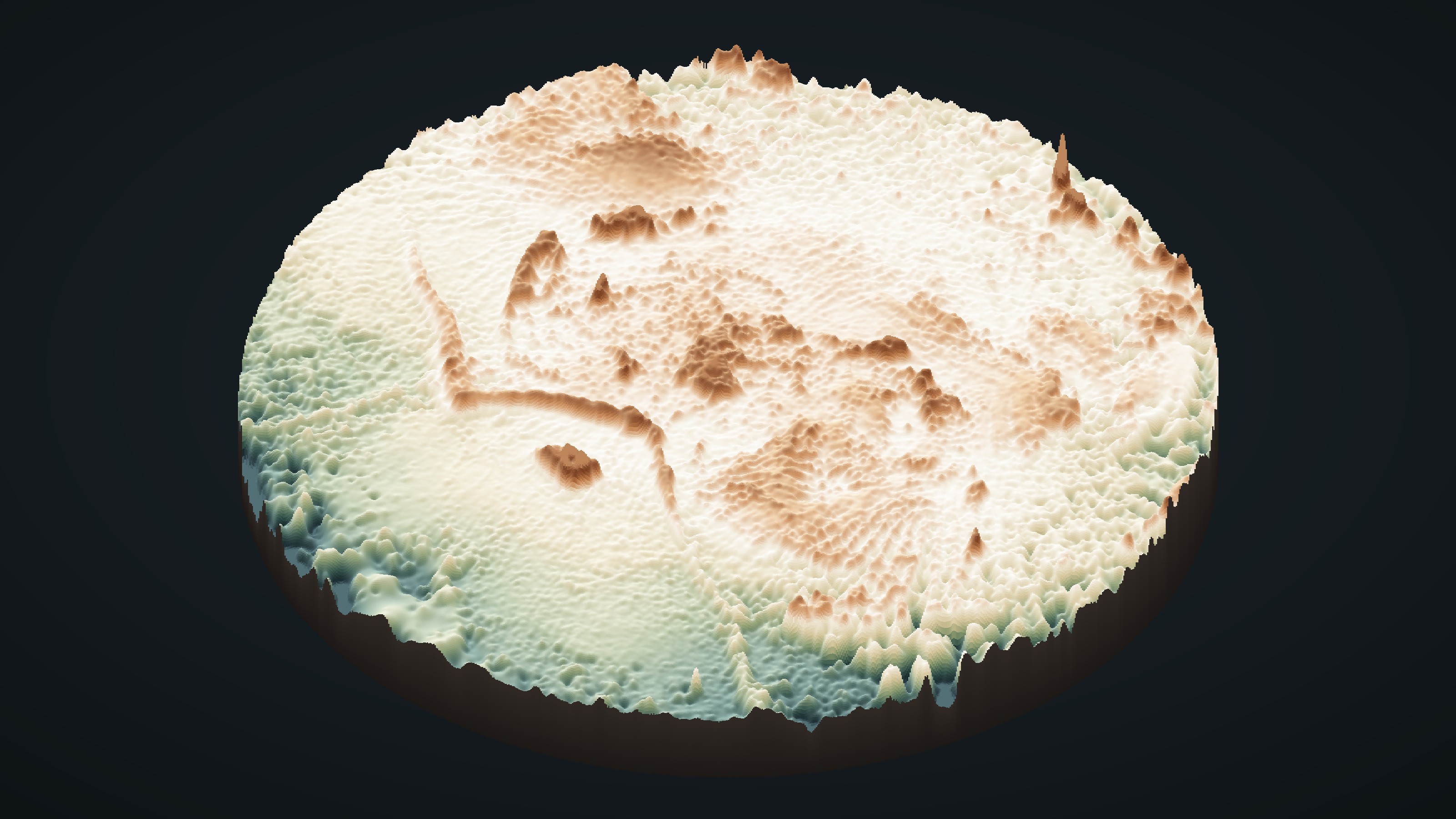
The central ~140 m of the survey rendered as a 3D surface. The smooth sinter terrace and the raised vent area stand out in the centre, with rougher ground toward the edge of the scan.
Shaded-Relief Elevation Model
The full survey at its native 0.18 m resolution, with no smoothing. Inset B shows a 20 × 20 m area at one-cell detail, so the true grid resolution is visible.
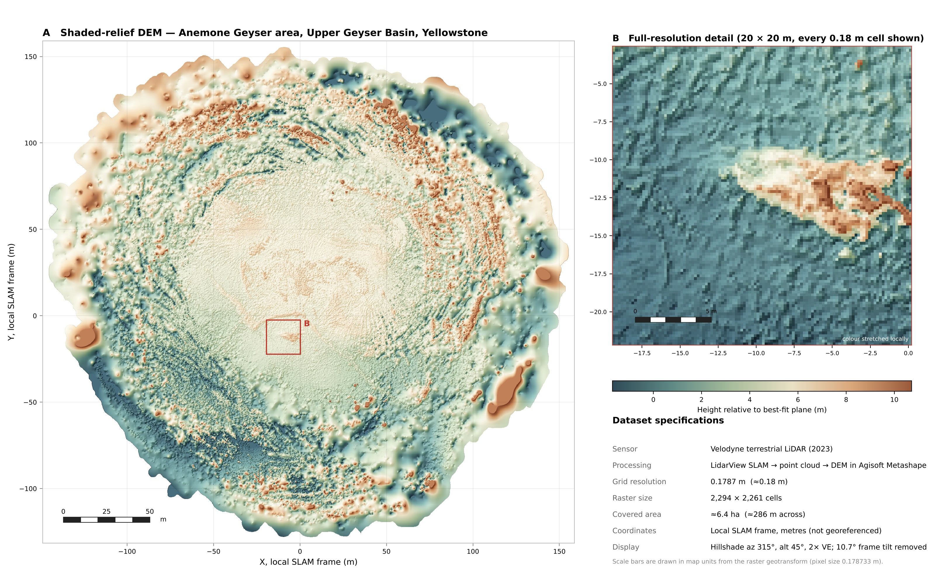
Reading it: a handheld scanner records its surroundings in its own tilted frame. I removed a 10.7° tilt by fitting a plane to the ground, so colour shows height above that plane rather than elevation above sea level. Scale bars are drawn from the raster's own cell size.
Processing Workflow
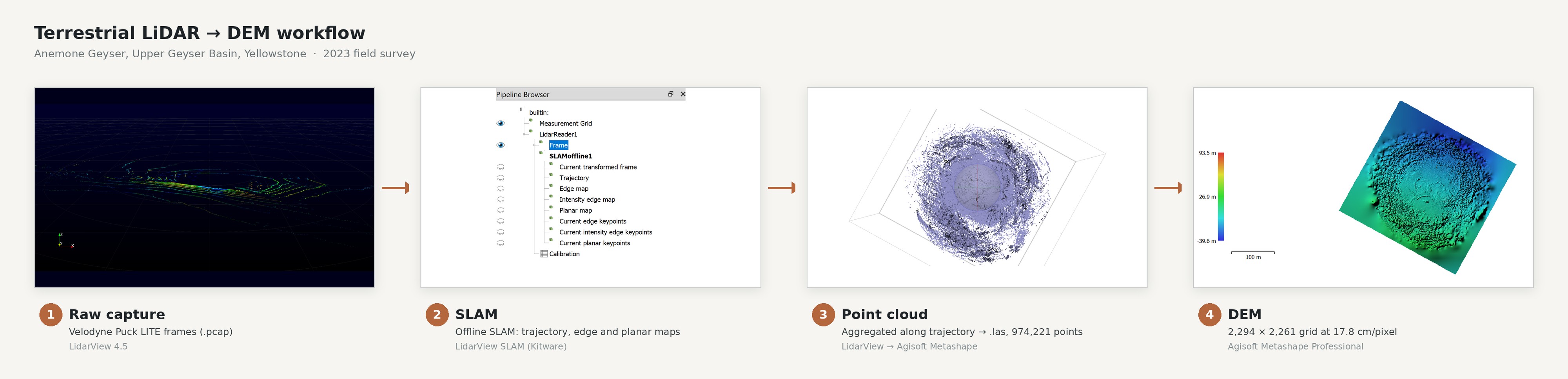
From raw sensor frames to a DEM, shown with screenshots from the actual processing of this dataset. The handheld scanner had no GPS, so SLAM recovers the scanner's path from the shape of the scene itself, and every frame is then placed along that path.
Vent Close-Up, 2022 iPad Capture
The previous season's dataset: a close-range scan of the Anemone vent collected by students with an iPad. It is the earlier of the two seasons in the intended time series, levelled and rendered for this portfolio.
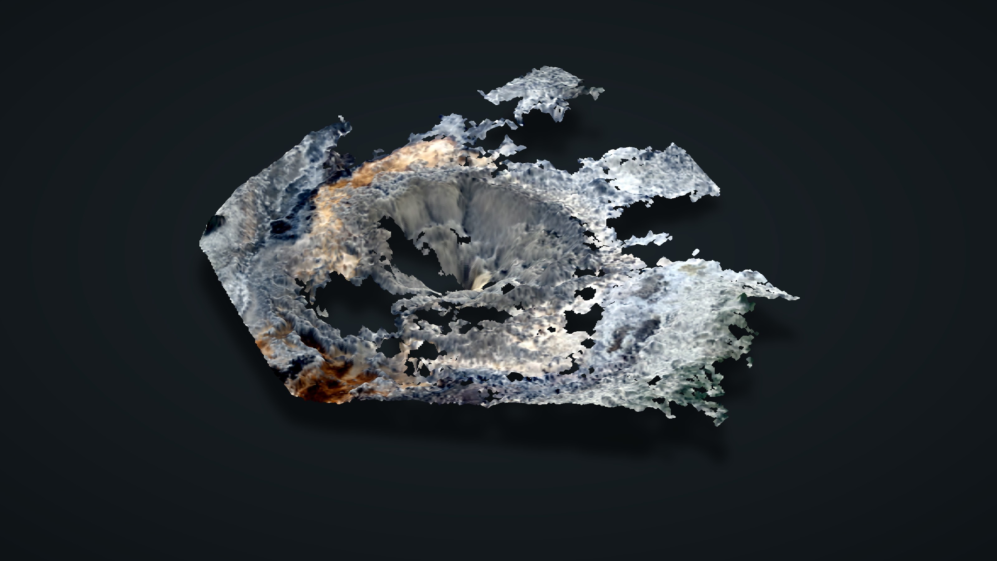
About the gaps: the students were learning to scan, so coverage is uneven and some surfaces were not captured. The gaps are left as they are rather than filled in, and the model has no surveyed scale reference, so no scale bar is shown.
Limitations
Both seasons were captured by students learning the equipment, with no ground control. The two datasets use different sensors, sit in separate local coordinate frames and share no reference points, so they can't yet be compared directly to measure geyser change. The DEM file also carries a UTM zone 12N label from the processing software even though its coordinates are local; it should be relabelled as a local coordinate system before reuse.
Next Steps: A Repeatable Change-Detection Survey
How I would complete the course leader's original goal if the field program resumed. Each step depends on the one before it.
- 1
Set ground control
Install and GNSS-survey a few permanent control points around each geyser, outside the active discharge area, so every season can be placed in the same real-world coordinate system.
- 2
Standardise the capture
Use the same scanner, pole height, walking route and pace every year, written into a field checklist. Review coverage on site before leaving so gaps are rescanned the same day.
- 3
Georeference each season
Process each capture through the existing SLAM workflow, then transform it onto the control points and record the fit error, so each point cloud carries a known accuracy.
- 4
Align on stable ground
Fine-align the seasons on terrain that should not change, away from the vent, so remaining differences reflect the geyser and not the survey.
- 5
Measure change
Compare seasons with M3C2 cloud-to-cloud distances, and report only changes larger than the combined survey error.
- 6
Deliver change maps
Produce maps of surface rise and loss for each geyser, with volume estimates and a short report that can be repeated each season.